Pathtracer (Part 1)

In this project:

• Raytracing to produce realistic renders of scenes with point or area lights and Lambertian surfaces.
• Optimization with bounding volume hierarchies and adaptive sampling.

Part 1: Ray Generation and Scene Intersection.

To generate a camera ray, I first calculate the coordinates of the lower left corner of the virtual camera sensor, as well as the width and height of the sensor rectangle. Then, I can convert from the given normalized image space coordinates \((x, y)\) to the coordinates \((xCamera, yCamera)\) in camera-space using scale proportions. I use the camera’s position and the camera-to-world rotation matrix to transform the ray’s origin and direction to world-space. After normalizing the ray’s direction vector, I return a new ray with the world-space origin and direction, with the minimum and maximum \(t\) values set to nClip and iClip.

To raytrace a single pixel in the rendering pipeline, I generate num_samples camera rays and use Monte Carlo estimation to estimate the integral of radiance over the given pixel. I sample from a uniform distribution over a unit square and add the random sample to the bottom left corner of the pixel \((x, y)\) to get a random point inside the pixel. I generate the camera ray corresponding to this random point and add its radiance contribution to my Monte Carlo estimator. After all num_samples samples, I update the pixel’s value in the sample buffer.

To test for intersection of a ray with a primitive, I substitute the ray equation \(O + td\) into the implicit formula of the geometric object (which could be a triangle or a sphere) and solve for the value of \(t\). For my triangle intersection algorithm, I use the Möller-Trumbore Algorithm to optimize solving for the intersection point. If the computed value of \(t\) lies within the ray’s range of \([min\_t, max\_t]\) and each coordinate-value of the intersection point’s barycentric coordinates is in the range \([0, 1]\), then the ray intersects the triangle. In the case of intersection, I update the Intersection data object accordingly.

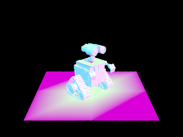
Images with normal shading for a few small .dae files.

Part 2: Bounding Volume Hierarchies

For my BVH construction algorithm, I first compute the bounding box of the given list of primitives and initialize a BVHNode with the bounding box. If the number of objects in the node is less than or equal to the max_leaf_size, the node is a leaf and I return it. Otherwise, I recursively build the left and right children.

The heuristic I use for the splitting point is the average of centroids along the longest axis of the bounding box. I find the longest axis by examining the bounding box’s extent member. Then, I sort the primitives according to which side of the splitting point they fall on, by iterating through the primitives and swapping elements by keeping track of a pointer to the end of the left child’s elements. If all the elements are sorted into one child, I decide that the node is a leaf node and terminate early.

Images with normal shading for a few large .dae files, rendered with BVH acceleration.

For cow.dae, BVH acceleration yields a speed-up factor of approximately 300, while for more complex scenes like beast.dae and maxplanck.dae, BVH acceleration is over 1000 times faster. For a complex geometric scene like CBlucy.dae, BVH acceleration can complete a render in just 0.0732 sec (I did not attempt to render CBlucy.dae without acceleration).

Part 3: Direct Illumination

For uniform hemisphere lighting, I take num_samples number of samples (equal to the number of lights times the number of samples per area light) over the unit hemisphere. Then, I trace a ray from point p in the sampled direction and check if this new ray intersects another object. I get the emission value of the surface at the new point of intersection, which is non-zero if the new ray intersects a light source. Then, using the reflectance value the estimate of incoming light, I can use the reflection equation to calculate the amount of outgoing light with a Monte Carlo estimator. After adding up the contributions from all the sampled directions, I normalize by dividing by the number of samples and dividing by the value of the probability density function, which is \(1 / 2\pi\) since we sample over the unit hemisphere.

Images rendered with both implementations of the direct lighting function.

Here is CBbunny.dae rendered with 1, 4, 16, and 64 light rays and with 1 sample per pixel using importance light sampling. As the number of samples per area light increases, the soft shadows become less noisy. At 1 or 4 light rays, the shadows under the bunny look very spotty. At 16 light rays, the shadows looks less like individual dots.

Uniform hemisphere sampling is somewhat slower than importance light sampling. For example, to render the Cornel Box bunny with 64 camera rays per pixel and 32 samples per area light, uniform hemisphere sampling takes about 98 seconds, while importance sampling takes 84 seconds. However, importance sampling greatly reduces the noise levels when compared to uniform hemisphere sampling at the same sample rates.

For example, when rendering the Cornel Box bunny with a very low sampling rate (1 camera ray per pixel and 1 sample per area light), the image created with uniform hemisphere sampling is so noisy that the shape of the model is barely visible, and the scene is barely lit. In contrast, the image created with importance sampling is much clearer.

Part 4: Global Illumination

For indirect lighting, I first add the direct illumination from one bounce radiance to L_out. Then, I sample one direction over the unit hemisphere in object space. I cast a ray from the given point hit_p in the sampled direction. Before checking for any intersections, I compute the continuation probability, the \(cpdf\). The \(cpdf = 1\) if this is the first bounce and the maximum ray depth is greater than 1; we should trace at least one indirect bounce regardless of Russian roulette. Otherwise, if the current ray depth is greater than 1 but this is not the first bounce, we terminate with probability 0.3, so the \(cpdf = 0.7\). If we do not terminate, I check for an intersection between the new sample ray and another scene object. If there is an intersection, I recurse with the new ray and new intersection point, then multiply by the reflectance and a cosine term, and normalize by both the \(pdf\) and the \(cpdf\). I add the contributed radiance to L_out and return L_out.

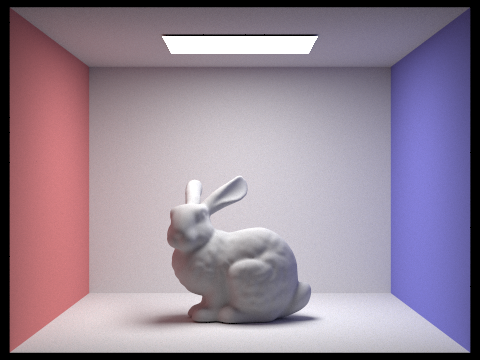
Some images rendered with global illumination using 1024 samples per pixels, 32 light rays per pixel, and maximum ray depth of 5.

The bunny, rendered with only direct illumination and then only indirect illumination, using 1024 samples per pixel.

Direct illumination only includes zero-bounce lighting and one-bounce lighting, so we see the rectangular area light on the ceiling of the Cornell Box and the first bounce of light from the bunny/walls to the camera. The shadows are completely black and the ceiling is not illuminated.

Only indirect illumination includes two or more bounces of light from the area light to the camera. The underside of the bunny and the ceiling of the Cornell Box are illuminated. The image is not very bright overall.

For CBbunny.dae, here are rendered views with max ray depth set to 0, 1, 2, 3, and 100. I used 1024 samples per pixel and 32 light rays per pixel.

A max ray depth of 0 corresponds to only zero-bounce lighting, so the only thing we see is the direct light from the area light. A max ray depth of 1 corresponds to only direct illumination. For any max ray depth greater than 1, I always calculate at least one additional indirect bounce. As max ray depth increases, the scene also gets slightly brighter.

Here is CBbunny.dae rendered with various sample-per-pixel rates: 1, 2, 4, 8, 16, 64, and 1024. I used 4 light rays and max ray depth of 5.

As the number of samples per pixel, the scene becomes less noisy. At just 1 sample per pixel, the image is very spotty, and the shadows on the bunny are not uniform. At 1024 samples per pixel, the image is much clearer, and the bunny’s shading is much smoother.

Part 5: Adaptive Sampling

Adaptive sampling is a technique used to reduce rendering times by taking fewer samples for pixels that converge more quickly, instead of sampling every single pixel a fixed number of times.

Each time I sample a pixel, I compute the illuminance from the radiance and track running totals for the sum of illuminances and the sum of squared illuminances. Every batch of samples, I calculate the mean and standard deviation of the illuminance samples so far. Then, I calculate the value of \(I\) and check if it is less than or equal to the max tolerance times the mean. If so, then this pixel has converged early. I stop sampling the pixel and update the sample buffer with the estimated radiance and sample count buffer with the total number of samples (less than the maximum possible number of samples).

Here are CBspheres_lambertian.dae and CBbunny.dae rendered with 2048 samples per pixel, 1 light ray, and max ray depth of 5. In the sampling rate image, red indicates that the pixel’s value did not converge early, while blue indicates that the pixel’s value converged early at a low sampling rate.